논문 링크 : https://papers.nips.cc/paper/5423-generative-adversarial-nets
Abstract
We simultaneously train two models: a generative model G that captures the data distribution, and a discriminative model D that estimates the probability that a sample came from the training data rather than G. The training procedure for G is to maximize the probability of D making a mistake.
Introduction
In the proposed adversarial nets framework, the generative model is pitted against an adversary: a discriminative model that learns to determine whether a sample is from the model distribution or the data distribution.
- generative model은 sample이 model distribution으로부터 왔는지 data distribution으로부터 왔는지 결정하는 discriminative model과 경쟁한다.
The generative model can be thought of as analogous to a team of counterfeiters, trying to produce fake currency and use it without detection, while the discriminative model is analogous to the police, trying to detect the counterfeit currency.
생성 모델은 위조 화폐를 만들어 탐지하지 않고 사용하려는 위조 팀과 유사하다고 생각할 수 있으며, 판별 모델은 위조 통화를 탐지하려는 경찰과 유사합니다.
→ 이러한 과정은 서로가 서로를 improve함.
In this article, we explore the special case when the generative model generates samples by passing random noise through a multilayer perceptron, and the discriminative model is also a multilayer perceptron. We refer to this special case as adversarial nets.
Minimax Game : 최악의 경우(max)를 가정했을 때, 손실(loss)을 최소화(min) 하는 것을 수학적으로 Minimax Game이라고 한다.
위폐를 찾는 경찰에 대해서 생각해보자
→ 무조건 위폐라고 답하는 경우: 위페와 지폐가 무작위하게 주어지므로, 테스트 횟수가 많아질 수록 정답을 맞힐 확률은 0.5에 가까워진다.
→ 무조건 진폐라고 답하는 경우: 마찬가지 이유로 정답을 맞힐 확률은 0.5에 가까워진다.
→ 무작위하게 답하는 경우: 지폐 한 장의 위조 여부를 맞힐 확률이 0.5이므로, 테스트 전체의 확률도 0.5에 가까워진다.
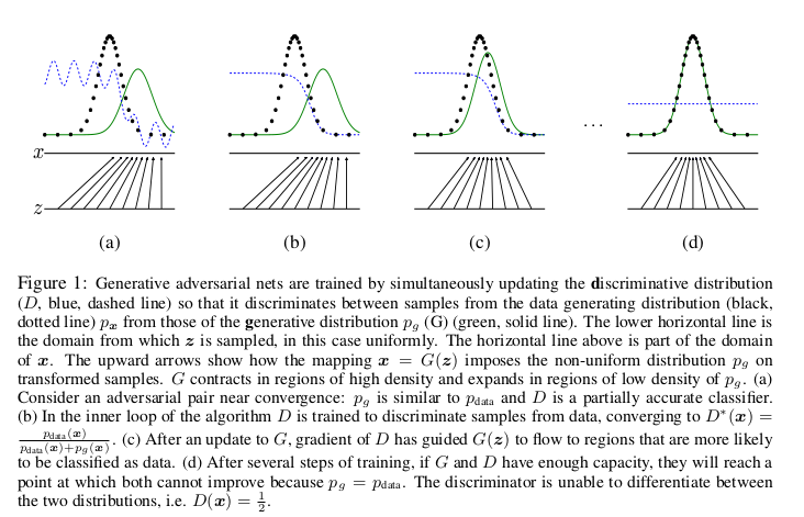
- 이에 대해 추가 설명, G가 너무 완벽하게 잘 만들어서 어떤게 진짜인지 구분할 수 없을 경우, D의 값은 1/2에 가까워 질 것이다. 따라서 D(G(z))가 1/2일 경우 학습은 종료된다.
3. Adversarial nets
To learn the generator’s distribution over data x, we define a prior on input noise variables , then represent a mapping to data space as , where G is a differentiable function represented by a multilayer perceptron with parameters .
- data x에 대한 generator의 distribution 를 학습시키기 위해, 논문에서는 입력 노이즈 변수 를 사전 정의 했다. 그리고 data space로의 mapping을 로 표현하였는데, 여기서 G는 파라미터 를 포함하는 multilayer perceptron에 의해 표현되는 미분 가능한 함수이다.
We also define a second multilayer perceptron that outputs a single scalar. represents the probability that x came from the data rather than .
We train D to maximize the probability of assigning the correct label to both training examples and samples from G. We simultaneously train G to minimize . In other words, D and G play the following two-player minimax game with value function :
- D가 training examples과 G로부터의 samples에 correct label을 잘 할당하는 것에대한 확률을 최대화 시키도록 D를 훈련시킨다. 동시에, G는 log(1-(D(G(z)))가 최소화 되도록(D가 잘 틀리도록(G에 의해 생성되는 데이터인 G(z)를 discriminate 했을 때, 이를 D가 1에 가깝게 되도록하면 잘 학습된 것으로 판단) 훈련시킨다. 이를 수식으로 표현하면 다음과 같다.

- 위의 Loss에 대해 부가 설명을 하자면 다음과 같다. 오른쪽 식을 maximize하는 D, 오른쪽 식을 minimize하는 G에 대한 내용이다. 먼저 앞의 기댓값에 대해, logD(x)는 x가 data로 부터 나왔기 때문에 D가 1의 값에 가깝게 나오도록 해야한다. 따라서 이는, D가 오른쪽 식을 maximize 해야한다. (0에 가까워지면 무한대로 가깝게 작아지므로.) 두 번째, 오른쪽에 대한 내용이다. D는 G(z)가 가짜 데이터임을 잘 맞춰야 하므로 D(G(z))가 0에 가깝게 나와야 한다. 따라서, log(1-D(G(z)))가 maximize하게끔 D를 잡아줘야 한다. G는 D가 G(z) 데이터가 실제 데이터인 것처럼 착각하게 만들어야 하므로, D(G(z))가 1에 가깝게 나오게끔 해주어야 한다. 따라서, 이 때, 1-D(G(z)) ⇒ 0 에 가깝게 나와야 하므로, 기댓값을 최소화 시키는 G가 필요한 것이다.
In the next section, we present a theoretical analysis of adversarial nets, essentially showing that the training criterion allows one to recover the data generating distribution as G and D are given enough capacity, i.e., in the non-parametric limit.
Optimizing D to completion in the inner loop of training is computationally prohibitive, and on finite datasets would result in overfitting. Instead, we alternate between k steps of optimizing D and one step of optimizing G. This results in D being maintained near its optimal solution, so long as G changes slowly enough. The procedure is formally presented in Algorithm1.
- 훈련의 내부 루프에서 완료까지 D를 최적화하는 것은 계산적으로 금지되어 있으며 finite datasets에서는 과적합이 발생할 수 있다. 대신, 우리는 D를 최적화하는 k 단계와 G를 최적화하는 한 단계를 번갈아 가며 진행한다. G가 충분히 천천히 변하는 한 D는 최적 솔루션 근처에서 유지됩니다. 절차는 Algorithm1에 공식적으로 나와 있다.
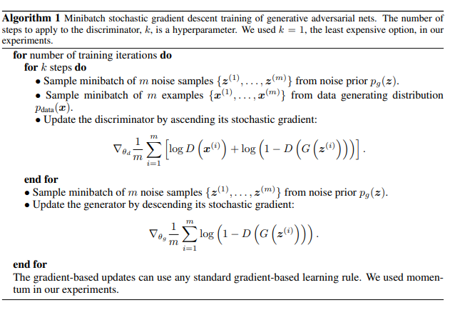
- Loss에서 discriminator는 maximize 해야 하기 때문에, stochastic gradient의 ascending을 통해 update를 하고, 반대로 generator는 minimize해야 하기 때문에 descending 해야한다고 생각.
In practice, equation 1 may not provide sufficient gradient for G to learn well. Early in learning, when G is poor, D can reject samples with high confidence because they are clearly different from the training data.
- 실제로는 equation 1이 G가 잘 학습되게끔 하는 적절한 gradient를 제공할 수 없을 수도 있다.
- 학습 초기에 Generate가 잘 안되면 Discriminate가 높은 확률로 samples를 잘 reject한다. → G(D(Z)) 가 0에 가까워짐.
- 논문에서 한 가지 실용적인 tip이 나오는데, 위에 value function에서 log(1−D(G(z))) 부분을 G 에 대해 minimize하는 대신 log(D(G(z))) 를 maximize하도록 G 를 학습시킨다는 것이다. 나중에 저자가 밝히 듯이 이 부분은 전혀 이론적인 동기로부터 추론을 한 것이 아니라 순수하게 실용적인 측면에서 적용을 하게 된 것 라 한다. 이유도 아주 직관적인데 예를 들어 학습 초기를 생각해보면, G 가 초기에는 아주 이상한 image들을 생성하기 때문에 D 가 너무도 쉽게 이를 real image와 구별하게 되고 따라서 log(1−D(G(z))) 값이 매우 saturate하여 gradient를 계산해보면 아주 작은 값이 나오기 때문에 학습이 엄청 느리다. 하지만 문제를 G= 로 바꾸게 되면, 초기에 D 가 G 로 나온 image를 잘 구별한다고 해도 위와 같은 문제가 생기지 않기 때문에 원래 문제와 같은 fixed point를 얻게 되면서도 stronger gradient를 줄 수 있는 상당히 괜찮은 해결방법이다.
4. Theoretical Results
The generator G implicitly defines a probability distribution as the distribution of the samples G(z) obtained when . Therefore, we would like Algorithm 1 to converge to a good estimator of , if given enough capacity and training time.
- generator G는 암묵적으로 확률분포 를 일 때 얻은 샘플 G(z)의 분포로서 정의한다. 따라서, 충분한 용량과 훈련 시간이 주어진다면 알고리즘 1이 의 좋은 estimator로 수렴되기를 바란다.
We will show in section 4.1 that this minimax game has a global optimum for . We will then show in section 4.2 that Algorithm 1 optimizes Eq 1, thus obtaining the desired result.
4.1 Global Optimality of
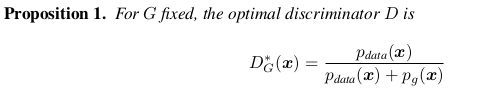
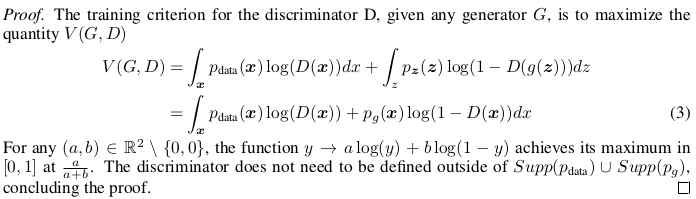
- Discriminator D의 훈련 기준은 어떤 generator G에 대해서든 V(G, D)의 quantity를 maximize 하는 것이다. 아래는 V(G, D)에 대한 식.
- 이에 대해서, 에서 어떤 (a, b) ((0,0)은 아님)에 대해, y = a*log(y) + b*log(1-y)가 에서 maximum 값을 가지는 것을 이용하면, optimal discriminator의 식을 이해 가능하다.
- 아래는 Optimal Discriminator D를 이용한 식 변환.
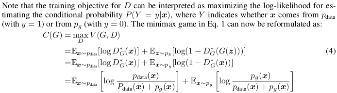
- D에 대한 훈련 목표는 조건부 확률 P(Y = y|x)를 추정하기 위한 log-likelihood를 최대화하는 것으로 해석될 수 있다. 여기서 Y는 x가 (y = 1 사용)에서 또는 (사용 y = 0).
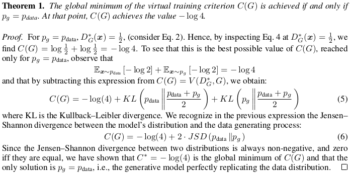
- virtual training criterion C(G)의 global minimum은 일 경우에 달성된다. 그 시점에서 C(G) 값은 -log 4 이다.
- 그냥 이런식으로 솔루션은 일 때가 유일함을 보이는 것이다.
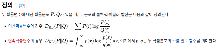
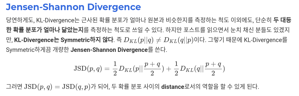
- 출처 : 위키피디아
4.2 Convergence of Algorithm 1
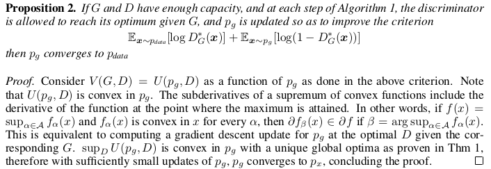
- G와 D가 충분한 용량을 갖고 있다면, Algorithm 1의 각 스텝에서 discriminator는 주어진 G에 대해 optimum에 다가가도록 한다. 그리고 는 기준(loss인 것 같음)을 상향시키기 위해 업데이트 된다. 그러면 는 에 수렴한다.
- 결국 이 Proposition이 뜻하는 바는, 수렴성에 대한 이야기이다. 중간에 In other words부터 보면, 만약 f(x)가 sup 이고, f_a(x)가 모든 a에 대해 x에서 convex일 때~~
- 아마 여러함수 f_i 전부가 convex function이다. 추가적인 해석 필요.
In practice, adversarial nets represent a limited family of distributions via the function G(z; ), and we optimize rather than itself, so the proofs do not apply. However, the excellent performance of multilayer perceptrons in practice suggests that they are a reasonable model to use despite their lack of theoretical guarantees.
- 실제로, adversarial nets은 분포에 대한 제한된 family를 function G를 통하여 표현하고 우리는 보다 를 optimize 하기 때문에 증명 적용이 잘 안된다. 그러나 MLP의 뛰어난 성능은 모델이 이론적인 guarantees가 부족함에도 사용하기에 reasonable 하다는 것을 제안한다.
5. Experiments
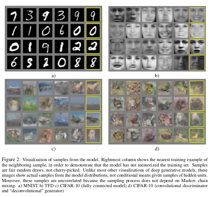
We trained adversarial nets an a range of datasets including MNIST[21], the Toronto Face Database (TFD) [27], and CIFAR-10 [19].
- dataset 설명
The generator nets used a mixture of rectifier linear activations(ReLU) [17, 8] and sigmoid activations, while the discriminator net used maxout [9] activations. Dropout [16] was applied in training the discriminator net. While our theoretical framework permits the use of dropout and other noise at intermediate layers of the generator, we used noise as the input to only the bottommost layer of the generator network.
- Network setting
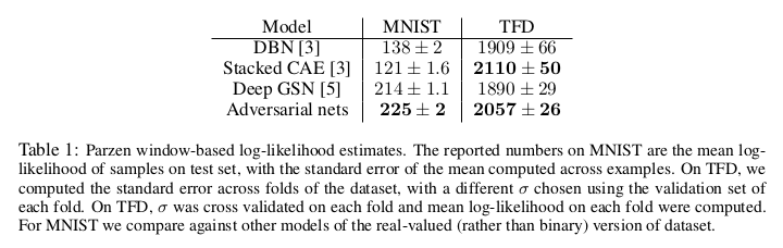
We estimate probability of the test set data under p g by fitting a Gaussian Parzen window to the samples generated with G and reporting the log-likelihood under this distribution. The σ parameter of the Gaussians was obtained by cross validation on the validation set.
6. Advantages and disadvantages
- Disadvantage
The disadvantages are primarily that there is no explicit representation of (x), and that D must be synchronized well with G during training (in particular, G must not be trained too much without updating D, in order to avoid “the Helvetica scenario” in which G collapses too many values of z to the same value of x to have enough diversity to model ), much as the negative chains of a Boltzmann machine must be kept up to date between learning steps.
- Advantage
The advantages are that Markov chains are never needed, only backprop is used to obtain gradients, no inference is needed during learning, and a wide variety of functions can be incorporated into the model.
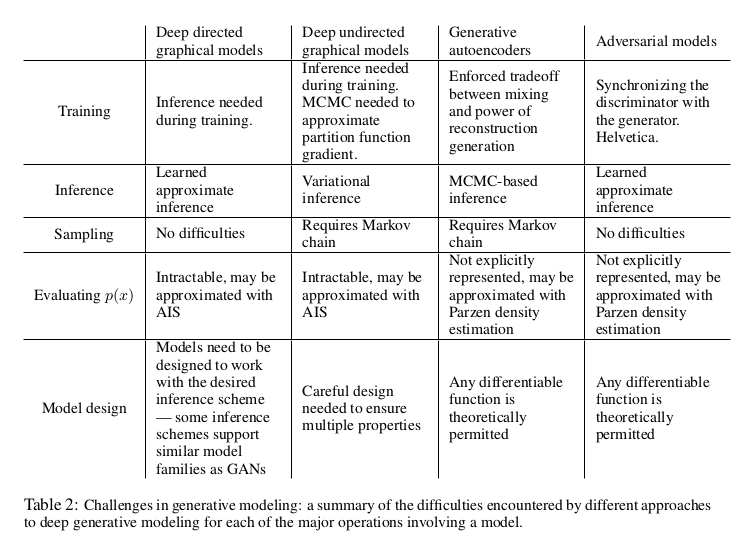
- Table 2 summarizes the comparison of generative adversarial nets with other generative modeling approaches.
Adversarial models may also gain some statistical advantage from the generator network not being updated directly with data examples, but only with gradients flowing through the discriminator. This means that components of the input are not copied directly into the generator’s parameters. Another advantage of adversarial networks is that they can represent very sharp, even degenerate distributions, while methods based on Markov chains require that the distribution be somewhat blurry in order for the chains to be able to mix between modes.
7. Conclusions and future work
- A conditional generative model p(x | c) can be obtained by adding c as input to both G and D.
- Learned approximate inference can be performed by training an auxiliary network to predict z given x. This is similar to the inference net trained by the wake-sleep algorithm [15] but with the advantage that the inference net may be trained for a fixed generator net after the generator net has finished training.
- One can approximately model all conditionals p(x S | x 6 S ) where S is a subset of the indices of x by training a family of conditional models that share parameters. Essentially, one can use adversarial nets to implement a stochastic extension of the deterministic MP-DBM [10].
- Semi-supervised learning: features from the discriminator or inference net could improve performance of classifiers when limited labeled data is available.
- Efficiency improvements: training could be accelerated greatly by devising better methods for coordinating G and D or determining better distributions to sample z from during training.
- 학부생 때 만든 것이라 오류가 있거나, 설명이 부족할 수 있습니다.
Uploaded by N2T
'Paper Summary' 카테고리의 다른 글
| Occupancy Networks: Learning 3D Reconstruction in Function Space, CVPR’19 (1) | 2023.03.26 |
|---|---|
| Deep Marching Cubes: Learning Explicit Surface Representations, CVPR’18 (0) | 2023.03.26 |
| DCGAN, ICLR’16 (0) | 2023.03.26 |
| Graph Attention Networks, ICLR’18 (0) | 2023.03.26 |
| GaAN: Gated Attention Networks for Learning on Large and Spatiotemporal Graphs, UAI’18 (0) | 2023.03.26 |
