논문 링크 : http://www.auai.org/uai2018/proceedings/papers/139.pdf
1. Introduction
Treating each attention head equally loses the opportunity to benefit from some attention heads which are inherently more important than others. To this end, we propose the Gated Attention Networks(GaAN) for learning on graphs. GaAN uses a small convolutional subnetwork to compute a soft gate at each attention head to control its importance.
Unlike the traditional multi-head attention that admits all attended contents, the gated attention can modulate the amount of attended content via the introduced gates.
Moreover, since only a simple and light-weighted subnetwork is introduced in constructing the gates, the computational overhead is negligible and the model is easy to train.
Furthermore, since our proposed aggregator is very general, we extend it to construct a Graph Gated Recurrent Unit (GGRU), which is directly applicable for spatiotemporal forecasting problem.
In summary, our main contributions include:
(a) a new multi-head attention-based aggregator with additional gates on the attention heads;
(b) a unified framework for transforming graph aggregators to graph recurrent neural networks;
(c) the state-of-the-art prediction performance on three real-world datasets.
2. Notations
We denote a single fully-connected layer with a non-linear activation α(·) as (x) = α(Wx + b), where θ = {W, b} are the parameters. Also, θ with different subscripts mean different transformation parameters.
For activation functions, we denote h(·) to be the LeakyReLU activation (Xu et al., 2015a) with negative slope equals to 0.1 and σ(·) to be the sigmoid activation.
(x) means applying no activation function after the linear transform.
We denote ⊕ as the concatenation operation and as sequentially concatenating through .
We denote the Hadamard product as ‘◦’ and the dot product between two vectors as <ㆍ,ㆍ>.
4. Gated Attention Networks
Generic formulation of graph aggregators
Given a node i and its neighboring nodes , a graph aggregator is a function in the form of , where and are the input and output vectors of the center node i.
is the set of the reference vectors in the neighboring nodes and Θ is the learnable parameters of the aggregator. In this paper, we do not consider aggregators that use edge features. However, it is straightforward to incorporate edges in our definition by defining to contain the edge feature vectors .
4.1 Multi-Head Attention Aggregator
We linearly project the center node feature x i to get the query vector and project the neighboring node features to get the key and value vectors.
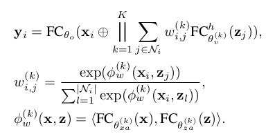
Here, K is the number of attention heads. is the k-th attentional weights between the center node i and the neighboring node j, which is generated by applying a softmax to the dot product values.
, and are the parameters of the kth head for computing the query, key and value vectors, which have dimensions of , and respectively.
The K attention outputs are concatenated with the input vector and pass to an output fully-connected layer parameterized by to get the final output , which has dimension .
The difference between our aggregator and that in GAT (Veličković et al., 2018) is that we have adopted the key-value attention mechanism and the dot product attention while GAT does not compute additional value vectors and uses a fully-connected layer to compute .
4.2 Gated Attention Aggregator
We compute an additional soft gate between 0 (low importance) and 1 (high importance) to assign different importance to each head.
In combination with the multi-head attention aggregator, we get the formulation of the gated attention aggregator:
- Multi-head attention aggregator는 center node와 그에 해당하는 neighborhood 사이의 여러 표현 부분 공간을 탐색 하지만 이 모두가 똑같이 중요하지는 않음. 그래서 추가적인 soft gate를 사용하여 각 head 마다 다른 importance를 부여함.
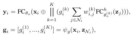
where is a scalar, the gate value of the k-th head at node i.
To make sure adding gates will not introduce too many additional parameters, we use a convolutional network that takes the center node and neighboring node features to generate the gate values.
There are multiple possible designs of the network. In this paper, we combine average pooling and max pooling to construct the network. The detailed formula is given below:
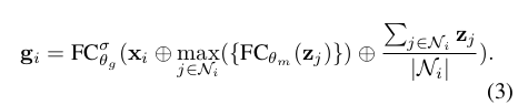
Here, maps the neighbor features to a dimensional vector before taking the element-wise max and maps the concatenated features to the final K gates. By setting a small , the subnetwork for computing the gate will have negligible computational overhead.
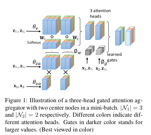
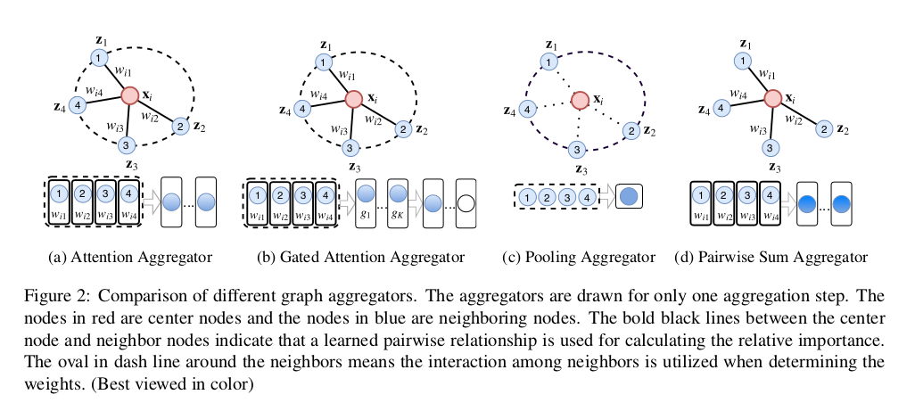
-The oval in dash line around the neighbors means the interaction among neighbors is utilized when determining the weights.
⇒ 이웃 주변의 점선 타원은 가중치를 결정할 때 이웃 간의 상호 작용을 활용함을 의미합니다.
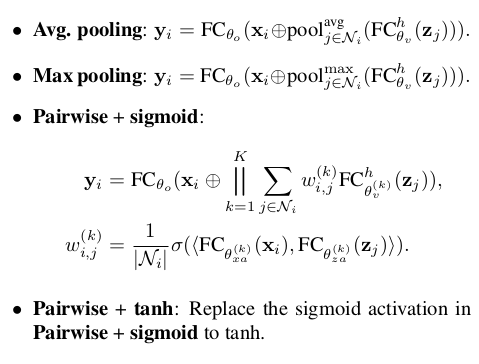
4.3 Other Graph Aggregators
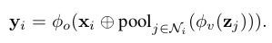
Graph pooling aggregators
The main characteristic of graph pooling aggregators is that they do not consider the correlation between neighboring nodes and the center node.
Instead, neighboring nodes’ features are directly aggregated and the center node’s feature is simply concatenated or added to the aggregated vector and then passed through an output function :
Graph pairwise sum aggregators
Like attention-based aggregators, graph pairwise sum aggregators also aggregate the neighborhood features by taking K weighted sums.
The difference is that the weight between node i and its neighbor j is not related to the other neighbors in . The formula of graph pairwise sum aggregator is given as follows:
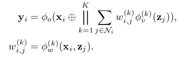
Here, is only related to the pair and while in attention-based models is related to features of all neighbors .
Baseline aggregators
To fairly evaluate the effectiveness of GaAN against previous work, we choose two representative aggregators in each category as baselines:
5. Inductive Node Classification
5.1 Model
During training, the validation and testing nodes are not observable and the goal is to predict the labels of the unseen testing nodes.
With a stack of M layers of graph aggregators, we will first sample a mini-batch of nodes and then recursively expand to be by sampling the neighboring nodes of .
The node representations, which are initialized to be the node features, will be aggregated in reverse order from to .
The representations of the last layer, i.e., the final representations of the nodes in , are projected to get the output.
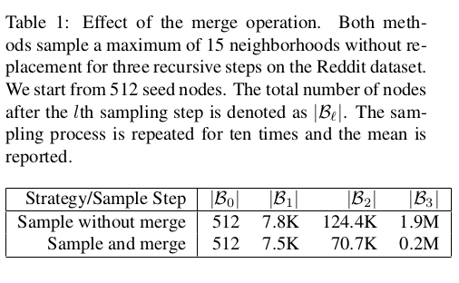
We only sample a subset of the neighborhoods for each node.
In our implementation, at the l-th sampling step, we sample min neighbors without replacement for the node i, where is a hyperparameter that controls the maximum number of sampled neighbors at the l-th step.
Moreover, to improve over GraphSAGE and further reduce memory cost, we merge repeated nodes that are sampled from different seeds’ neighborhoods within each mini-batch.
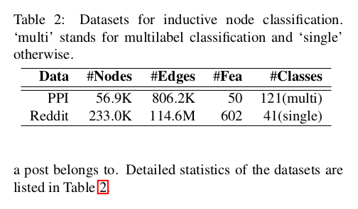
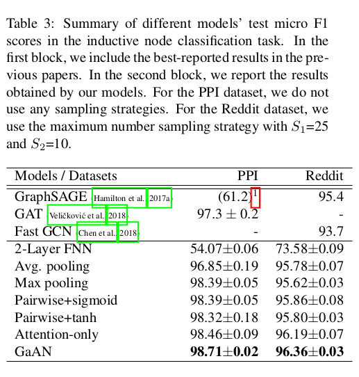
5.2 Experimental Setup
5.5 Ablation Analysis
Effect of the number of attention heads and the sample size
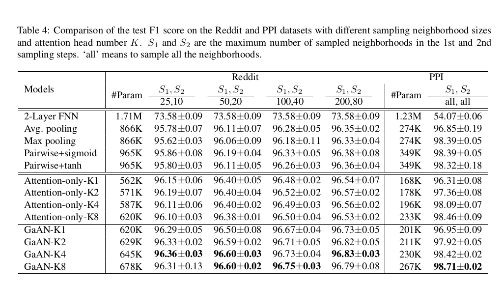
K : head number , S_1 and S_2 : maximum number of sampled neighborhoods in the 1st and 2nd sampling steps , all : sample all the neighborhoods
Effect of output dimensions in the PPI dataset
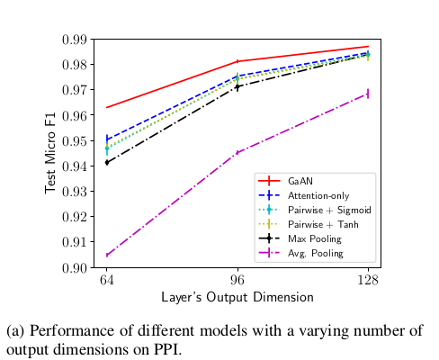
We find that the performance becomes better for larger output dimensions and the proposed GaAN consistently outperforms the other models.
Visualization of gate values
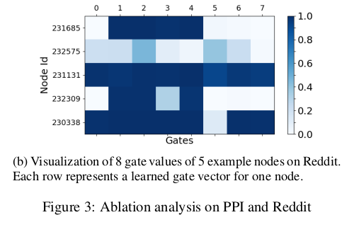
It illustrates the diversity of the learned gate combinations for different nodes.
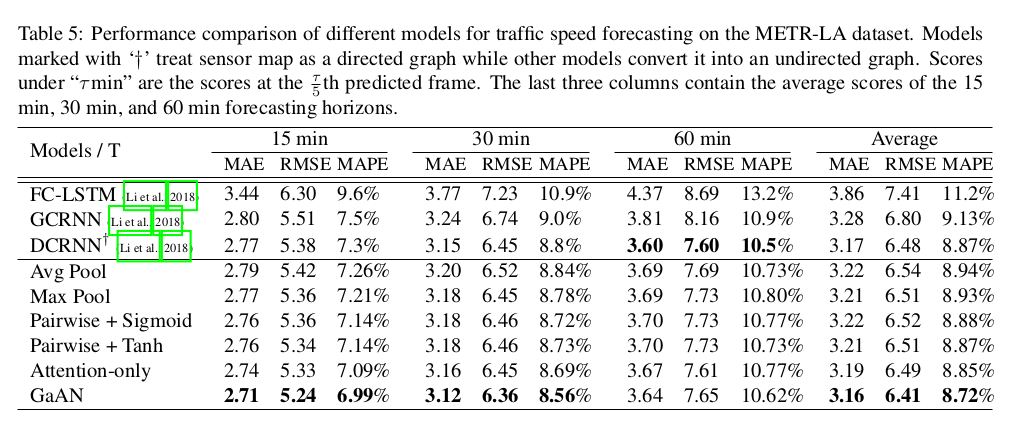
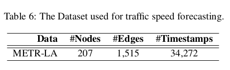
6. Traffic Speed Forecasting
We formulate traffic speed forecasting as a spatiotemporal sequence forecasting problem where the input and the target are sequences defined on a fixed spatiotemporal graph, e.g., the road network.
To simplify notations, we denote as applying the aggregator for all nodes in G, i.e., .
Based on a given graph aggregator Γ, we can construct a GRU-like RNN structure using the following equations:

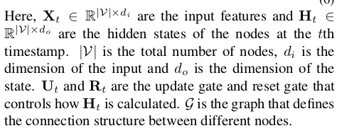
Predict the future K steps of traffic speeds in the sensor network , ,..., based on the previous J steps of observed traffic speeds , , ..., .
7. Conclusion and Future Work
We introduced the GaAN model and applied it to two challenging tasks:
(1) inductive node classification and traffic speed forecasting. GaAN beats previous state-of-the-art algorithms in both cases. In the future, we plan to extend GaAN by integrating edge features and processing massive graphs with millions or even billions of nodes.
(2) Moreover, our model is not restricted to graph learning. A particularly exciting direction for future work is to apply GaAN to natural language processing tasks like machine translation.
- 학부생 때 만든 것이라 오류가 있거나, 설명이 부족할 수 있습니다.
Uploaded by N2T
'Paper Summary' 카테고리의 다른 글
| DCGAN, ICLR’16 (0) | 2023.03.26 |
|---|---|
| Graph Attention Networks, ICLR’18 (0) | 2023.03.26 |
| Learning Actor Relation Graphs for Group Activity Recognition, CVPR’19 (0) | 2023.03.26 |
| Mesh Graphormer, ICCV’21 (0) | 2023.03.26 |
| Actor-Transformers for Group Activity Recognition, CVPR’20 (0) | 2023.03.26 |