DG-STGCN: Dynamic Spatial-Temporal Modeling for Skeleton-based Action Recognition, ACM MM’22

 

논문 링크 : https://arxiv.org/pdf/2210.05895.pdf

Abstract

We note that existing GCN based approaches primarily rely on prescribed graphical structures (i.e., a manually defined topology of skeleton joints), which limits their flexibility to capture complicated correlations between joints. To move beyond this limitation, we propose a new framework for skeleton-based action recognition, namely Dynamic Group Spatio-Temporal GCN (DG-STGCN). It consists of two modules, DG-GCN and DG-TCN, respectively, for spatial and temporal modeling. In particular, DG-GCN uses learned affinity matrices to capture dynamic graphical structures instead of relying on a prescribed one, while DG-TCN performs group-wise temporal convolutions with varying receptive fields and incorporates a dynamic joint-skeleton fusion module for adaptive multi-level temporal modeling.

• 기존의 GCN-based method는 주로 규정된 graphical structure에 의존하므로 joint간의 복잡한 correlation을 capture하는 유연성이 제한된다. 이러한 limitation을 뛰어넘기 위해서 skeleton-based action recognition을 위한 새로운 framework인 Dynamic Group Spatio-Temporal GCN (DG-STGCN)을 제시한다. 이는 DG-GCN과 DG-TCN이라는 spatial, temporal modeling을 위한 2가지의 module로 이루어져있다. 특히, DG-GCN은 규정된 것에 의존하는 대신 학습된 affinity matrix를 사용하여 dynamical graphical structure를 캡처하는 반면, DG-TCN은 다양한 receptive field로 group-wise temporal convolution을 수행하고 adaptive multi-level temporal modeling을 위한 dynamic joint-skeleton fusion module을 통합한다.

 

1. Introduction

We propose a novel GCN architecture for skeleton-based action recognition, namely DG-STGCN. It enables group-wise dynamic spatial-temporal modeling for skeleton data. In DG-STGCN, spatial modeling and temporal modeling are performed separately by dynamic group GCNs (DG-GCNs) and dynamic group temporal ConvNets (DG-TCNs), respectively. Our proposed framework has three appealing properties. First, DG-STGCN is purely based on learnable coefficient matrices for spatial modeling, eliminating the cumbersome procedure to define a good joint topology manually. Second, the dynamic group-wise design enables the dynamic spatial temporal modeling of the skeleton motion with diversified groups of graph convolutions and temporal convolutions, improving the representation capability and flexibility. Third, DG-STGCN achieves significant improvements on multiple benchmarks while preserving the model efficiency.

• 저자는 skeleton-based action recognition을 위한 새로운 GCN architecture인 DG-STGCN을 제안한다. 이는 skeleton data에 대한 group-wise dynamic spatial-temporal modeling을 가능하게 한다. DG-STGCN에서 spatial modeling과 temporal modeling은 각각 dynamic group GCN(DG-GCNs)과 dynamic group temporal ConvNets (DG-TCNs)에 의해 별도로 수행된다. 저자가 제시한 framework는 3가지의 특성을 가지고 있다.

• (1) DG-STGCN은 spatial modeling을 위한 순수하게 학습가능한 coefficient matrix를 기반으로 하므로 joint topology를 manually define 해야하는 번거로운 절차가 필요하지 않다.

• (2) Dynamic group-wise design은 다양한 group의 graph convolution과 temporal convolution으로 skeleton motion에 대한 dynamic spatial-temporal modeling을 가능하게 하여 capability와 flexibility를 향상시킨다.

• (3) DG-STGCN은 model efficiency를 유지하면서 여러 benchmark에서 상당한 개선을 달성한다.

 

3. DG-STGCN

3.1. ST-GCN Recap

Notation

For inputs and intermediate features$\mathbf{X}\in {\mathbf{R}}^{T\times V\times C}$ of a GCN for skeleton processing, T denotes the temporal length; V denotes the number of skeleton joints; C denotes the number of channels (if X is the input, C is usually 2 or 3).

For coefficient matrices$\mathbf{A}\in {\mathbf{R}}^{K\times V\times V}$ used for spatial modeling, K denotes the number of matrices (we also call it the number of groups). We use$\mathcal{F}$ to denote the GCN block;$\mathcal{G},\mathcal{T}$ to indicate the spatial module and temporal module, respectively.

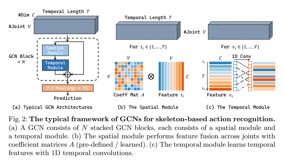
In skeleton-based action recognition, GCN approaches take a sequence of human joint coordinates (a T × V × C tensor$\mathbf{X}$ for each person) as input and predict the action category. Figure 2 provides a quick recap of ST-GCN, an early and representative work for skeleton-based action recognition. ST-GCN utilizes stacked N GCN blocks (N = 10) to process the coordinate tensors. A GCN block F consists of two components: a spatial module G and a temporal module T. Given a skeleton feature$\mathbf{X}\in {\mathbf{R}}^{T\times V\times C}$ , G first performs channel inflation and reshaping to get a 4D tensor${\mathbf{X}}^{\prime }\in {\mathbf{R}}^{T\times K\times V\times C}$ , and then uses a set of coefficient matrices$\mathbf{A}$ for inter-joint spatial modeling.

• Skeleton-based action recognition에서 GCN은 human joint coordinate의 sequence(T × V × C tensor$\mathbf{X}$ for each person)를 input으로 받아 action category를 예측한다. Fig.2는 대표적인 model인 ST-GCN의 요약을 제시한다. ST-GCN은 10개의 GCN block을 활용해 coordinate tensor를 처리한다. GCN block$\mathcal{F}$ 는 2개의 component로 이루어져있는데, spatial module$\mathcal{G}$ temporal module$\mathcal{T}$ 이다. Skeleton feature$\mathbf{X}\in {\mathbf{R}}^{T\times V\times C}$ 가 주어지면$\mathcal{G}$ 는 channel inflation과 reshaping을 통해 4D tensor${\mathbf{X}}^{\prime }\in {\mathbf{R}}^{T\times K\times V\times C}$ 를 얻는다. 그리고 inter-joint spatial modeling을 위해 coefficient matrices$\mathbf{A}$ 를 사용한다.

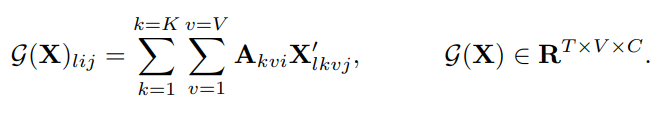
The output of$\mathcal{G}$ is further processed by$\mathcal{T}$ to learn temporal features. The computations of F can be summarized as:

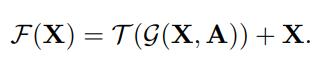
Specifically, ST-GCN [53] adopts sparse matrices derived from a prescribed graphical structure (weighted by learnable importance scores) as A, and instantiates$\mathcal{T}$ with a single 1D temporal convolution (kernel size 9).

• 구체적으로, ST-GCN은 규정된 graphical structure에서 파생된 sparse matrix를 (learnable importance score를 통해 weighted 됨.) A로 사용하고, single 1D temporal convolution (kernel size 9)를 통해$\mathcal{T}$ 를 인스턴스화 한다.

 

3.2. DG-GCN: Dynamic Spatial Modeling from Scratch

The spatial module$\mathcal{G}$ fuses features of different joints with coefficient matrices$\mathbf{A}$, while the final recognition performance is highly dependent on the choice of$\mathbf{A}$. One common practice in previous works is to first set$\mathbf{A}$ as a series of manually defined sparse matrices (derived from the adjacency matrix of joints) and learn a refinement$\Delta \mathbf{A}$ during model training [5,39,41].$\Delta \mathbf{A}$ can be either static, as a trainable parameter, or dynamic, generated by the model depending on the input sample. Though intuitive, we argue that this paradigm is limited in flexibility and may lead to inferior recognition performance than purely data-driven approaches.

• Spatial module$\mathcal{G}$ 는 coefficient matrices$\mathbf{A}$ 와 서로 다른 joint의 feature를 융합하는 반면, 최종적인 recognition performance는$\mathbf{A}$ 의 선택에 크게 의존한다. 이전 work에서의 일반적인 관행은 먼저$\mathbf{A}$ 를 수동으로 정의하는 sparse matrix (joint adjacency matrix로 부터 파생됨)로 설정하고 모델 학습 중에 개선된$\Delta \mathbf{A}$를 학습하는 것이다.$\Delta \mathbf{A}$는 학습 가능한 파라미터로 input sample에 따라 static하거나 dynamic할 수 있다. 저자는 이 패러다임이 flexibility에 제한이 있고 순전히 data-driven한 방식보다 recognition 성능이 떨어질 수 있다고 주장한다.

Thus we make the coefficient matrices A fully learnable. In DG-GCN,$\mathbf{A}\in {\mathbf{R}}^{K\times V\times V}$ is a learnable parameter rather than a set of manually defined matrices. For initialization, instead of resorting to derivations of the adjacency matrix, we directly initialize A with normal distribution. With random initialization, K can be set to an arbitrary value, enabling the novel multi-group design in DG-GCN.

• 따라서, 저자는 coefficient matrix A를 fully learnable하게 만들었다. DG-GCN에서$\mathbf{A}\in {\mathbf{R}}^{K\times V\times V}$는 manually defined matrix가 아닌 학습 가능한 파라미터이다. Initialization을 위해 A를 직접 normal distribution으로 초기화한다. 이러한 초기화를 통해 K를 임의의 값으로 설정할 수 있어 (adjacency가 아니므로 group을 여러개 둘 수 있음.) DG-GCN에서 새로운 multi-group의 design이 가능하다.

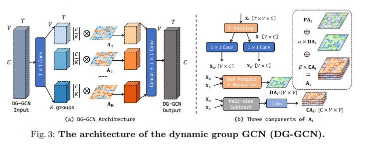
We demonstrate the architecture of DG-GCN in Figure 3(a). In DG-GCN, the coefficient matrices A consist of K different components (K = 8 in experiments). The input (with C channels) is first processed with a 1 × 1 convolution, to generate K feature groups (each with$[\frac{C}{K}]$ channels). We then perform spatial modeling for each feature group independently with the corresponding${\mathbf{A}}_i$. Finally, K feature groups are concatenated along the channel dimension and then processed by another 1 × 1 convolution to generate the output.

• Figure 3(a)에서 DG-GCN의 architecture를 보여준다. DG-GCN에서 coefficient matrices$\mathbf{A}$ 는 K개의 다른 component로(K = 8) 구성된다. Input (C channel의)은 먼저 1 x 1 convolution을 통과해서 K개의 feature group을 생성한다. (각 channel은$[\frac{C}{K}]$.) 그 다음 해당하는${\mathbf{A}}_i$ 와 독립적으로 각 feature group에 spatial modeling을 수행한다. 마지막으로 K개의 feature group이 channel dimension을 따라 contact된 다음 또 다른 1 x 1 convolution을 통과해 output을 생성한다.

Each coefficient matrix${\mathbf{A}}_i$ consists of three learnable components. First, a dataset-wise parameter${\mathbf{PA}}_i$ (the static term) is learned throughout training. Besides, we learn data-dependent refinements${\mathbf{DA}}_i$ and${\mathbf{CA}}_i$, serving as the dynamic terms. The two terms are different in that${\mathbf{DA}}_i$ is channel-agnostic while${\mathbf{CA}}_i$ is channel-specific. Figure 3(b) demonstrates how we obtain${\mathbf{DA}}_i$ and${\mathbf{CA}}_i$. Given the input feature$\mathbf{X}$, temporal pooling is first used to eliminate the dimension T. Two separate 1 × 1 convolutions are then applied to$\bar{\mathbf{X}}\in {\mathbf{R}}^{V\times C}$ to get${\mathbf{X}}_a\in {\mathbf{R}}^{V\times C}$ and${\mathbf{X}}_b\in {\mathbf{R}}^{V\times C}$, respectively.

• 각 coefficient matrix${\mathbf{A}}_i$ 는 3개의 learnable components로 구성된다. 먼저,${\mathbf{PA}}_i$ 는 dataset-wise parameter인데(static-term?) 학습을 통해서 만들어진다. (scratch상태에서 부터 학습됨) 그리고 data-dependent refinements인${\mathbf{DA}}_i$ 와${\mathbf{CA}}_i$ 도 학습한다. 이 두 개의 term 중${\mathbf{DA}}_i$ 는 channel-agnostic하고${\mathbf{CA}}_i$ 는 channel-specific하다. Figure. 3(b)는${\mathbf{DA}}_i$ 와${\mathbf{CA}}_i$ 를 얻는 방법을 보여준다. Input feature$\mathbf{X}$ 가 주어지면 temporal pooling을 통해서 Temporal dimension을 제거한다. 그리고 2개의 1 x 1 convolution을 적용해서 각각${\mathbf{X}}_a$ 와${\mathbf{X}}_b$ 를 얻어낸다.

${\mathbf{DA}}_i\in {\mathbf{R}}^{V\times V}$,${\mathbf{CA}}_i\in {\mathbf{R}}^{C\times V\times V}$

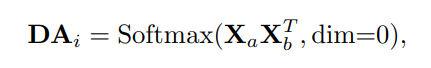
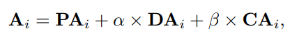
$\alpha ,\beta$ are two learnable parameters. In experiments, we find the term${\mathbf{PA}}_i$ plays the major role and cannot be omitted, while two dynamic terms also steadily contribute to the final recognition performance.

• $\alpha ,\beta$ 는 학습가능한 파라미터. 실험에서 term${\mathbf{PA}}_i$ 가 major role을 하고 생략불가능 하다는 것을 발견함. 나머지 2개의 dynamic term도 꾸준이 final recognition performance에 관여한다.

3.3. DG-TCN: Multi-group TCH with Dynamic Joint-Skeleton Fusion

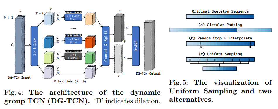
We also adopt the dynamic group-wise design in temporal modeling. Following [5,29], we first replace the vanilla temporal module with a multi-group TCN. As shown in Figure 4, a multi-group TCN consists of multiple branches with different receptive fields. Each branch performs temporal modeling for a feature group independently.

• 저자는 temporal modeling에서 dynamic group-wise design을 채택한다. 이전 work처럼 vanilla temporal module을 multi-group TCN으로 교체한다. Fig. 4에서 볼 수 있듯이 multi-group TCN은 각각 다른 receptive fields가 있는 여러 branch로 구성된다. 각 branch는 feature group에 대해 independent하게 temporal modeling을 수행한다.

We further propose to perform temporal modeling at both joint-level and skeleton-level parallelly. Thus we develop the D-JSF module for explicit modeling and dynamically fusing the joint-level and skeleton-level features. In D-JSF, we first perform average pooling to V joint-level features$\{{\mathbf{X}}_1,...,{\mathbf{X}}_V|{\mathbf{X}}_i\in {\mathbf{R}}^{C\times T}\}$ to obtain the skeleton-level feature$\mathbf{S}$. A multi-group TCN processes both the skeleton feature$\mathbf{S}$ and$V$ joint features${\mathbf{X}}_i$ in parallel to get${\mathbf{S}}^{\prime }$,${\mathbf{X}}_i^{\prime }$. Dynamic joint-skeleton fusion is then applied to merge${\mathbf{S}}^{\prime }$ into each${\mathbf{X}}_i^{\prime }$. Specifically, each DG-TCN instance contains a learned parameter$\gamma \in {\mathbf{R}}^V$. After the adaptive joint-skeleton fusion, the feature for joint i is${\mathbf{X}}_i^{\prime },{\gamma }_i{\mathbf{S}}^{\prime }$, which will be further processed with a 1 × 1 convolution. In practice, we find that the dynamic fusion with a learnable weight γ is the key to the success of DG-TCN.

• 저자는 joint-level 그리고 skeleton-level 모두에서 동시에 temporal modeling을 수행할 것을 제안한다. 따라서, joint level과 skeleton-level feature의 dynamically fusing과 explicit modeling을 위한 D-JSF module을 개발한다. D-JSF에서 먼저 skeleton-level feature S를 얻기 위해 joint-level feature$\{{\mathbf{X}}_1,...,{\mathbf{X}}_V|{\mathbf{X}}_i\in {\mathbf{R}}^{C\times T}\}$ 를 average pooling한다. multi-group TCN은${\mathbf{S}}^{\prime }$,${\mathbf{X}}_i^{\prime }$ 를 얻기 위해 skeleton feature$\mathbf{S}$ 와 V개의 joint feature${\mathbf{X}}_i$ 를 parallel 하게 처리한다.

• 여기서 더 자세하게 설명하자면,${\mathbf{X}}_i\in {\mathbf{R}}^{T\times V\times C}$ 를 V-dimension에서 average pooling 하면$\mathbf{S}\in {\mathbf{R}}^{T\times C}$ 의 skeleton-level feature를 얻을 수 있음. 이를 contact & split 과정을 통해${\mathbf{S}}^{\prime }$,${\mathbf{X}}_i^{\prime }$ 를 얻음.

• 그런 다음${\mathbf{S}}^{\prime }$ 를${\mathbf{X}}_i^{\prime }$ 에 병합하기 위해 dynamic joint-skeleton fusion이 적용된다. 특히, 각 DG-TCN instance에는 learnable parameter$\gamma \in {\mathbf{R}}^V$ 가 포함된다. Adaptive joint-skeleton fusion후에 joint i에 대한 feature는${\mathbf{X}}_i^{\prime },{\gamma }_i{\mathbf{S}}^{\prime }$ 이고 이는 1 x 1 convolution으로 추가 처리된다. 실제로 저자는 learnable weight$\gamma \in {\mathbf{R}}^V$ 와의 dynamic한 fusion이 DG-TCN의 성공의 key임을 발견했다.

• Joint skeleton fusion → 이전 논문을 보니 약간 separate한 two-stream framework를 사용해서 얻은 feature를 잘 합치는 과정을 이야기하는 것 같음.

 

3.4. Uniform Sampling as Temporal Data Augmentation

• 이전 논문처럼 Uniform Sampling이 action recognition을 위해 더 도움이 된 다는 것을 보임.

 

4. Experiment

4.1 Datasets

Top-1 accuracy on NTURGB+D and Kinetics-400;

report the Mean Top-1 accuracy for BABEL and Toyota SmartHome.

 

4.2. Implementation Details

• DG-STGCN은 ST-GCN의 기본 설정을 따른다. 10개의 GCN block이 있고 각 GCN block은 DG-GCN과 DG-TCN으로 구성됨. 기본 channel width는 64. 5, 8번쨰 GCN block에서 temporal pooling을 수행해서 temporal length를 절반으로 줄이고 channel width도 2배로 늘린다.

 

4.3. Ablation Study

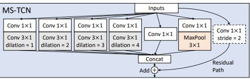
Our baseline uses GCN with randomly initialized coefficient matrices (3 components) for spatial modeling and a multi-branch TCN (with six branches: 4 kernel-3 1D convolution branches with dilation [1, 2, 3, 4], a kernel-3 max-pooling branch, and a 1 × 1 convolution branch) for temporal modeling.

• Spatial modeling을 위해 random하게 initialization된 coefficient matrices (3 components)와 multi-branch TCN (4 kernel-3 1D convolution branches with dilation [1, 2, 3, 4], a kernel-3 max-pooling branch, and a 1 × 1 convolution branch)을 temporal modeling을 위해 사용한다. (여기서 kernel-3는 3x1 kernel인 것 같음.) → 이전 논문과 비슷하게 사용. Inception 처럼 사용하는것 같음.

 

Preliminary: Is a pre-defined topology indispensable?(없어서는 안될?)

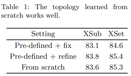
We consider three alternatives: 1). a fixed topology [39] which is pre-defined; 2). 1 with a static learnable refinement; 3). a topology learned from scratch, randomly initialized at the beginning. Table 1 shows that a learnable refinement largely improves the recognition performance. However, removing the pre-defined topology only leads to a moderate drop (≤ 0.2%). Following Occam’s Razor, we do not use any prescribed graphical structure in the following experiments. This opens a great design space for spatial GCNs.

• 규정된 graphical structure가 spatial modeling에 얼마나 중요한지 알아본다. 저자는 3가지의 대안을 고려했다. 1) Pre-defined topology 2) Static learnable refinement 3) Scratch로 부터 학습된 topology (무작위 초기화)

• Table 1은 learnable refinement가 recognition performance를 크게 향상시킨다는 것을 보인다.

• 아마 adjacency matrix를 학습가능하게 사용하는지 아닌지를 말하는 것 같음.

 

Dynamic Group GCN (DG-GCN).

Ablation on the group number.

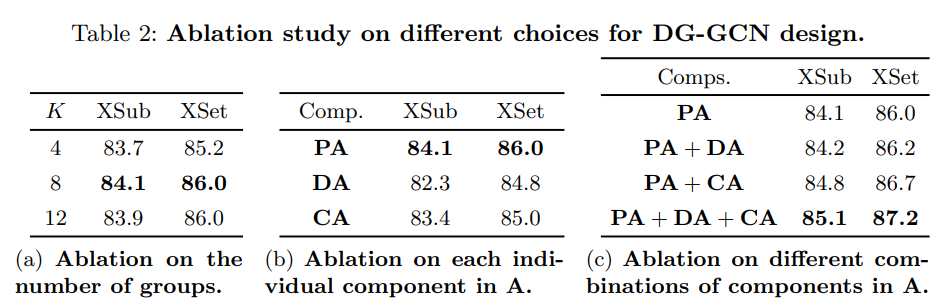
We first explore using different values for the hyper-parameter K, which is the number of groups in DG-GCN. We gradually increase K from 4 to 12 and list the recognition performance in Table 2a. More groups improve the flexibility of DG GCN and benefit the skeleton spatial modeling. Empirically, we find that eight groups lead to a reasonably good result (adding more groups does not help a lot). Thus we use eight groups in the following experiments.

• K 값에 대한 ablation study. K를 4에서 12로 점진적으로 증가시키고 이에 대한 recognition performance를 Table 2 (a)에 나열한다. 저자는 K=8일때 상당히 좋은 결과를 가져왔다는 것을 발견했다.

 

Ablation on the topology components.

As a network parameter, the learned from-scratch topology is a static component (PA) in the final coefficient matrices. In DG-GCN, we also incorporate two dynamic terms, namely DA (channel-agnostic) and CA (channel-specific). Two dynamic components share the same encoding layers (two 1×1 convolutions), which means all models with dynamic components share a similar parameter size (1.69M) and FLOPs (1.65G). Compared to using only the static component (1.25M params, 1.63G FLOPs), using dynamic terms increases the parameter size by 1/3, while the computation consumed almost remains the same. We first evaluate each component individually and show the recognition performance in Table 2b. Dynamic terms used alone cause severe degradation in recognition performance compared to the static term PA, which partially explains why previous purely dynamic approaches (like SGN [58]) can not beat the state-of-the-art. We further investigate the effects of different combinations of terms and present the results in Table 2c. For spatial modeling, the channel-specific term CA plays a more critical role than the channel-agnostic term DA. Combining three components leads to the best recognition results.

• Network parameter로서 scratch 상태에서부터 학습된 topology는 최종 coefficient matrices인 static component인 PA 이다. DG-GCN에서는 DA (channel-agnostic)과 CA(channel-specific)이라는 두 가지 dynamic term도 사용한다. 2개의 dynamic components는 동일한 encoding layer를 share한다. 각 구성요소에 대해 개별적으로 평가하고 recognition 성능을 표 2b에 표시한다. PA없이 단독으로 사용되는 dynamic term들은 성능이 심각하게 안좋아서 뺐다. Spatial modeling의 경우 CA는 DA보다 더 중요한 역할을 하고, 3가지를 동시에 사용할 경우 최상의 결과를 얻을 수 있다.

 

How much data does DG-GCN require?

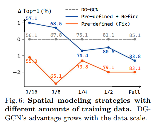
• DG-GCN을 학습하려면 얼마나 많은 데이터가 필요한지 궁금함. 그래서 학습에 사용되는 데이터 양을 선택함. Fig 6에서는 3가지의 spatial modeling 전략을 비교함. Pre-defined topolgy는 계속 안좋게 나옴. Training set이 작을 때, manually하게 정의된 topology는 skeleton data의 spatial modeling에 유리하다고 분석함. 그리고, 학습 데이터가 많을수록 유망함을 보여줌.

 

Dynamic Group TCN (DG-TCN)

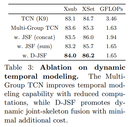
We conduct ablation experiments to validate our design choice for the temporal module. Instead of the vanilla implementation (a single 1D convolution with kernel 9) in ST GCN, we adopt the DG-TCN for temporal modeling. DG-TCN consists of multiple branches with different receptive fields for dynamic temporal modeling. It is also equipped with the dynamic joint-skeleton fusion module (D-JSF) for adaptive fusion between joint motion and skeleton motion. Table 3 shows that, besides improving the temporal modeling capability, the multi-group design also substantially reduces the computation cost by using a small channel width for every single branch. For the JSF module, besides fusing the skeleton-level feature with joint-level feature dynamically with learnable coefficients, we also test two simpler alternatives, e.g., directly concatenating or summing up the two features. From Table 3, we see that D-JSF performs the best among the three alternatives.

• Temporal module에 대한 design을 검증하기 위한 ablation study. ST-GCN의 vanilla implementation (kernel 9를 사용한 단일 1D convolution) 대신 temporal modeling을 위해 DG-TCN을 택한다. 이는 다른 receptive fields를 가지고 있는 multiple branch로 구성되어있고, joint motion과 skeleton motion의 adaptive fusion을 위한 D-JSF를 포함한다. Table 3에서 temporal modeling을 바꾼것 외에도 GFLOPs를 보면 TCN보다 낮다는 것을 볼 수 있다. (채널 폭이 작기 때문) JSF module의 경우 skeleton-level feature를 학습 가능한 coefficient를 사용하는 것 외에도 두 가지 feature를 concat하거나 sum하는 것과 같은 간단한 테스트를 포함한다. Table 3에서 저자는 D-JSF가 세 가지 대안 중 가장 좋은 성능을 보인다는 것을 알 수 있다.

 

Uniform Sampling as Temporal Data Augmentation.

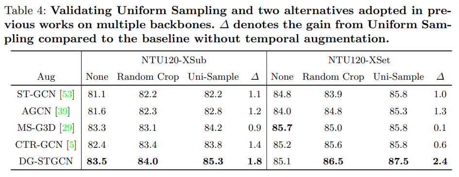
• Random Cropping이나 Uniform Sampling이 성능 향상에 도움이 됨.

 

4.4. Comparisons with the State-of-the-Art.

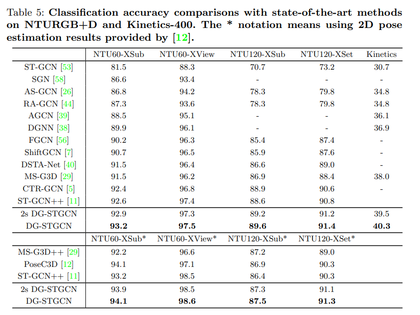
• 여러 데이터셋에서 전부 sota 달성. Fair한 비교를 위해 각 method들 마다 4가지 modality (joint, bone, joint motion, bone motion)를 input으로 사용해서 얻은 performance를 ensemble하여 reporting 하였다. 여기서, 2s DG-STGCN은 논문에서 제시한 joint + bone fusion을 사용한 방법인데, 이것만 해도 성능이 충분히 잘 나오는 것을 볼 수 있음. 위에는 2D pose를 기반으로 돌린 것.

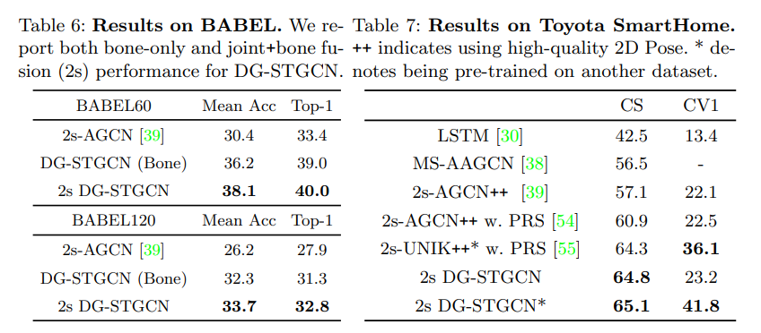
• BABEL dataset이랑 SmartHome dataset에서의 결과도 보여줌. CS와 CV1는 split의 이름이다.

 

5. Conclusion

This work presents a highly dynamic framework DG-STGCN for the spatial-temporal modeling of skeleton data. DG-STGCN consists of two novel modules with dynamic multi-group design, namely DG-GCN and DG-TCN. For spatial modeling, DG-GCN fuses joint-level features with coefficient matrices learned from scratch and does not rely on prescribed graphical structures. Meanwhile, DG-TCN adopts the group-wise temporal convolution with diversified receptive fields and the dynamic joint-skeleton feature module for dynamic multi-level temporal modeling. DG-STGCN surpasses the state-of-the-art on four challenging benchmarks, demonstrating its impressive capability and effectiveness.

• 본 논문은 skeleton data의 spatial-temporal modeling을 위한 dynamic framework인 DG-STGCN을 제시한다. DG-STGCN은 DG-GCN 및 DG-TCN이라는 dynamic multi-group design을 갖춘 두 개의 새로운 module로 구성된다. Spatial modeling의 경우 DG-GCN은 joint-level feature를 scratch상태에서 부터 학습한 coefficient matrices와 fusion하고 규정된 graphical structure에 의존하지 않는다. 한편 DG-TCN은 다양한 receptive field를 가진 group-wise temporal convolution과 dynamic multi-level temporal modeling을 위한 dynamic-skeleton feature module을 채택했다. DG-STGCN은 네 가지의 benchmark에서 sota의 성능과 효율성을 보여주었다.

 

Uploaded by

N2T