1. Introduction
- We present an end-to-end framework for recovering a full 3D mesh of a human body from a single RGB image. We use the generative human body model, SMPL, which parameterizes the mesh by 3D joint angles and a low-dimensional linear shape space.
- A key insight is that there are large-scale 2D keypoint annotations of in-the-wild images and a separate large-scale dataset of 3D meshes of people with various poses and shapes.
1.1 Contribution
- The idea is that, given an image, the network has to infer the 3D mesh parameters and the camera such that the 3D keypoints match the annotated 2D keypoints after projection.
2. To deal with ambiguities, these parameters are sent to a discriminator network, whose task is to determine if the 3D parameters correspond to bodies of real humans or not.
1.2 Approach
- We infer 3D mesh parameters directly from image features, while previous approaches infer them from 2D keypoints. This avoids the need for two stage training and also avoids throwing away valuable information in the image such as context. - 3D mesh parameters 를 directly 하게 image features로 부터 추론함. 이렇게 하면 two stage training 과 valuable information이 버려지는 것을 피할 수 있음.
- Going beyond skeletons, we output meshes, which are more complex and more appropriate for many applications. Again, no additional inference step is needed. - 더 복잡하고 많은 응용이 가능한 mesh를 출력함. 추가적인 추론 단계는 필요하지 않음.
- Our framework is trained in an end-to-end manner. We out-perform previous approaches that output 3D meshes [5, 20] in terms of 3D joint error and run time. - end-to-end 방법으로 훈련되었고, 3D mesh의 error와 run time 측면에서 더 뛰어남.
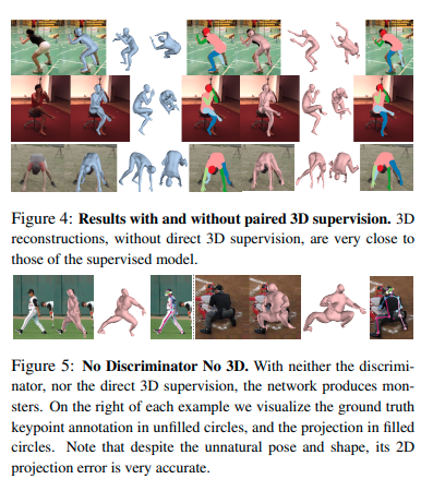
- We show results with and without paired 2D-to-3D data. Even without using any paired 2D-to 3D supervision, our approach produces reasonable 3D reconstructions. This is most exciting because it opens up possibilities for learning 3D from large amounts of 2D data. - paired 2D-to-3D data가 없더라도, 이런 접근 방법은 reasonable한 3D reconstruction을 생산해낸다.
3. Model
We propose to reconstruct a full 3D mesh of a human body directly from a single RGB image I centered on a human in a feedforward manner. During training we assume that all images are annotated with ground truth 2D joints.
- feedforward 방법으로 RGB 이미지로 부터 directly하게 human body에 대한 3D mesh를 reconsturction한다. 훈련 중에 우리는 모든 이미지가 2D joint GT가 labeling 되어있다는 가정을 한다.
Additionally we assume that there is a pool of 3D meshes of human bodies of varying shape and pose. Since these meshes do not necessarily have a corresponding image, we refer to this data as unpaired
- 다양한 자세와 모양의 3D meshes of human bodies가 매우 많다고 가정함. 이 mesh와 일치하는 이미지가 반드시 있지는 않기 때문에, 이 data를 unpaired라고 함.
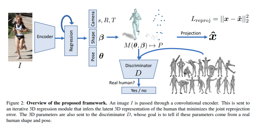
위 사진은 end-to-end 방식으로 train될 수 있는 network의 architecture를 보여준다.
Convolutional features of the image are sent to the iterative 3D regression module whose objective is to infer the 3D human body and the camera such that its 3D joints project onto the annotated 2D joints.
- 이미지의 Convolution feature는 3D human body와 camera를 추론하여 3D joint가 annotate된 2D joint에 projection 되도록하는 iterative한 3D regression module로 전송된다.
The inferred parameters are also sent to an adversarial discriminator network whose task is to determine if the 3D parameters are real meshes from the unpaired data.
- 추론된 parameters는 또한 adversarial discriminator network로 보내지는데 이 network는 unpaired data로 부터 이 3D parameter가 real meshes인지 아닌지를 결정한다.
This encourages the network to output 3D human bodies that lie on the manifold of human bodies and acts as a weak-supervision for in-the-wild images without ground truth 3D annotations.
- 이는 network가 3D human human bodies에 대한 manifold에 있는 3D human bodies를 출력하도록 encourage하고, in-the-wild image에 대해 3D annotation GT가 없어도 weak-supervision처럼 작동한다.
When ground truth 3D information is available, we may use it as an intermediate loss.

where λ controls the relative importance of each objective, 1 is an indicator function that is 1 if ground truth 3D is available for an image and 0 otherwise. We show results with and without the 3D loss. We discuss each component in the following.
- GT 3D 정보가 사용가능할 경우에 우리는 intermediate loss를 사용할 수 있음.
- 그래서 우리의 전반적인 목표는 다음과 같은 Loss로 볼 수 있는데, λ는 각각의 objective에 대한 relative importance를 조절하고, 1은 indicator function인데, 만약 GT가 사용가능 하다면 1, 아니면 0임.
3.1 3D Body Representation
We encode the 3D mesh of a human body using the Skinned Multi-Person Linear (SMPL) model.
SMPL is a generative model that factors human bodies
shape() : how individuals vary in height, weight, body proportions
- PCA shape space 에서 첫 번째 10개의 coefficients들만 뽑아냄.
pose() : how the 3D surface deforms with articulation (3D 표면이 관절(articulation)로 변형되는 방법)
- axis-angle representation에 대한 K = 23 joint의 relative 3D rotation으로부터 modeling 된다.
SMPL is a differentiable function that outputs a triangulated mesh with N = 6980 vertices,
M(θ, β) ∈ , which is obtained by shaping the template body vertices conditioned on β and θ, then articulating the bones according to the joint rotations θ via forward kinematics, and finally deforming the surface with linear blend skinning.
- 여기서 R에서 3이 곱해지는 이유는 각 vertices들의 (x, y, z)좌표가 들어가기 때문이라고 생각됨.
The 3D keypoints used for reprojection error, X(θ, β) ∈ , are obtained by linear regression from the final mesh vertices.
We employ the weak-perspective camera model and solve for the global rotation ∈ in axis-angle representation, translation(평행이동) t ∈ and scale s ∈ .
- 위의 s, t, R은 camera calibration과 관련이 있음.
Thus the set of parameters that represent the 3D reconstruction of a human body is expressed as a 85 dimensional vector Θ = {θ, β, R, t, s}.
Given Θ, the projection of X(θ, β) is

where Π is an orthographic projection.
- 3D → 2D projection
3.2 Iterative 3D Regression with Feedback
The goal of the 3D regression module is to output Θ given an image encoding φ such that the joint reprojection error is minimized.

Here ∈ is the ith ground truth 2D joints and ∈ {0,1}^k is the visibility (1 if visible, 0 otherwise) for each of the K joints.
- visibility는 projection후에 사진에서 실제로 보이는지 안보이는지에 대한 것이므로 보이면 1이다.
논문에서 directly하게 를 regressing 하는 것은 가 rotation parameters를 가지고 있어서 너무 어려우므로 iterative error feedback(IEF)를 통해 progressive changes를 만들어낸다고 함.
Specifically, the 3D regression module takes the image features φ and the current parameters Θ_t as an input and outputs the residual ∆Θ_t.
- 3D regression module은 image features와 current parameters를 input으로 받고 output으로 residual를 출력함.
The parameter is updated by adding this residual to the current estimate Θ_(t+1) = Θ_t + ∆Θ_t.
The initial estimate Θ_0 is set as the mean .
In this work, we keep everything in the latent space and simply concatenate the features [φ, Θ] as the input to the regressor.
- regressor의 input으로 다음 두 features를 concatenate한 것을 사용함.
Additional direct 3D supervision may be employed when paired ground truth 3D data is available.
- 추가적인 3D supervision은 paired 3D data GT가 사용 가능할 때 이용가능함.
Supervision in terms of SMPL parameters [β, θ] may be obtained through MoSh when raw 3D MoCap marker data is available.
- MoSh : motion and shape capture
- MoCap : motion capture

As noted by these approaches, supervising each iteration with the final objective forces the regressor to overshoot and get stuck in local minima.
Thus we only apply L_reproj and L_3D on the final estimate Θ_T , but apply the adversarial loss on the estimate at every iteration Θ_t forcing the network to take corrective steps that are on the manifold of 3D human bodies.
- 각 iteration 마다 supervising 하는 것은 local minima에 빠지게 하므로, L_reproj와 L_3D는 마지막 estimate 에만 적용시킨다. Adversarial loss는 매 iteration에 적용시키는데 이는 network가 올바른 3D human bodies가 있는 manifold로 이동하게 한다.
3.3 Factorized Adversarial Prior
We use a discriminator network D that is trained to tell whether SMPL parameters correspond to a real body or not. SMPL has a factorized form that we can take advantage of to make the adversary more data efficient and stable to train.
- network D의 역할과 SMPL의 장점.
More concretely, we mirror the shape and pose decomposition of SMPL and train a discriminator for shape and pose independently. The pose is based on a kinematic tree, so we further decompose the pose discriminators and train one for each joint rotation.
- SMPL을 이용하여 discriminator를 훈련시킨다.
This amounts to learning the angle limits for each joint.
- 이러한 learning이 angel limits를 얻게 해준다.
In order to capture the joint distribution of the entire kinematic tree, we also learn a discriminator that takes in all the rotations.
- entire kinematic tree에 대한 joint distribution을 얻기 위해 우리는 모든 rotation에서 얻어지는 discriminator를 훈련시킨다.
Since the input to each discriminator is very low dimensional (10-D for β, 9-D for each joint and 9K-D for all joints), they can each be small networks, making them rather stable to train. All pose discriminators share a common feature space of rotation matrices and only the final classifiers are learned separately.
- discriminator은 dimension이 매우 낮아서 networks가 매우 작고 그것이 train을 더 stable하게 만들어준다. 모든 pose discriminator는 공통 rotation matrices에 대한 feature space를 공유하고 finial classifier만 따로 훈련된다.
The importance of the adversarial prior is paramount when no paired 3D supervision is available. Without the adversarial prior the network produces totally unconstrained human bodies as we show in section 4.3.
- 대충 adversarial prior가 unconstrained human bodies를 안 만들어 내도록 규제한다는 뜻.
n all we train K + 2 discriminators. Each discriminator D_i outputs values between [0, 1], representing the probability that Θ came from the data. Let E represent the encoder including the image encoder and the 3D module.
- 여기서 K + 2 개의 discriminator가 있다는 뜻은, K개의 joint와 pose, shape를 각각 independently하게 train해서 그런 듯 함.
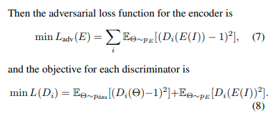
- 여기서 위의 L_adv(E)는 image를 Encoding하여 Discrimator에 집어 넣은 값이 1(세타가 data로 부터 왔다는 뜻)과 가까워 지도록 L를 minimize 한다. 여기서는 Encoder의 Loss이므로 Encoder가 최대한 Discriminator를 잘 속여야해서 1에 가깝게 나와야 함.
- 아래 L(D_i)는 Discriminator에 대한 loss이므로 이에 대해 설명하면, ~ 는 pose data로 부터 세타를 추출해냈고, 그 세타에대해 각각의 Discriminator 의 기댓값이 1에 가까워지도록 하는게 앞부분이다. ( 가 1에 가깝다는 뜻은, 세타가 실제 데이터로부터 왔다는 것을 의미함. 실제로 이 세타는 pose data로 부터 왔기 때문에 1에 가까워야 함.)
- 뒷 부분에서는 Discriminator가 E(I)가 prediction 되었다는 것을 최대한 잘 맞추어야 하기 때문에 E(I)의 discrimination 값이 0에 가까워 지도록 해야함.(E(I)는 prediction된 값이다.)
3.4 Implementation Details
The in-the-wild image datasets annotated with 2D keypoints that we use are LSP, LSP-extended MPII and MS COCO.
We filter images that are too small or have less than 6 visible keypoints and obtain training sets of sizes 1k, 10k, 20k and 80k images respectively. We use the standard train/test split of these datasets. All test results are obtained using the ground truth bounding box.
For the 3D datasets we use Human3.6M and MPIINF-3DHP.
We leave aside sequences from training Subject 8 of MPI-INF-3DHP as the validation set to tune hyper-parameters, and use the full training set for the final experiments.
Both datasets are captured in a controlled environment and provide 150k training images with 3D joint annotations.
For Human3.6M, we also obtain ground truth SMPL parameters for the training images using MoSh from the raw 3D MoCap markers.
The unpaired data used to train the adversarial prior comes from MoShing three MoCap datasets: CMU, Human3.6M training set and the PosePrior dataset, which contains an extensive variety of extreme poses. These consist of 390k, 150k and 180k samples respectively.
The definition of the K = 23 joints in SMPL do not align perfectly with the common joint definitions used by these datasets.
We follow and use a regressor to obtain the 14 joints of Human3.6M from the reconstructed mesh. In addition, we also incorporate the 5 face keypoints from the MS COCO dataset.
New keypoints can easily be incorporated with the mesh representation by specifying the corresponding vertex IDs1 . In total the reprojection error is computed over P = 19 keypoints.
Architecture
We use the ResNet-50 network for encoding the image, pretrained on the ImageNet classification task. The ResNet output is average pooled, producing features φ ∈ .
The 3D regression module consists of two fully-connected layers with 1024 neurons each with a dropout layer in between, followed by a final layer of 85D neurons. We use T = 3 iterations for all of our experiments.
- 85 dimension인 이유 : : 3K (69-dim) , : 10-dim , t : 2-dim , s : 1-dim, R : 3-dim
The discriminator for the shape is two fully-connected layers with 10, 5, and 1 neurons. For pose, θ is first converted to K many 3 × 3 rotation matrices via the Rodrigues formula. Each rotation matrix is sent to a common embedding network of two fully-connected layers with 32 hidden neurons. Then the outputs are sent to K = 23 different discriminators that output 1-D values
The discriminator for overall pose distribution concatenates all K ∗ 32 representations through another two fully-connected layers of 1024 neurons each and finally outputs a 1D value.
Experimental Setting
All layers use ReLU activations except the final layer. The learning rates of the encoder and the discriminator network are set to 1 × 10⁻⁵ and 1×10⁻⁴ respectively. We use the Adam solver and train for 55 epochs. Training on a single Titan 1080ti GPU takes around 5 days. The λs and other hyper-parameters are set through validation data on MPI-INF-3DHP dataset. Implementation is in Tensorflow.
4. Experimental Results
Although we recover much more than 3D skeletons, evaluating the result is difficult since no ground truth mesh 3D annotations exist for current datasets. Consequently we evaluate quantitatively on the standard 3D joint estimation task. We also evaluate an auxiliary task of body part segmentation.
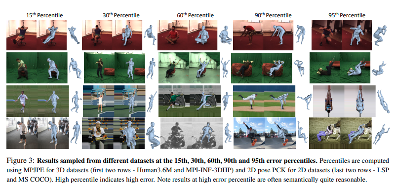
- error율이 높아도 충분히 reasonable한 결과를 얻을 수 있음.
4.1 3D Joint Location Estimation
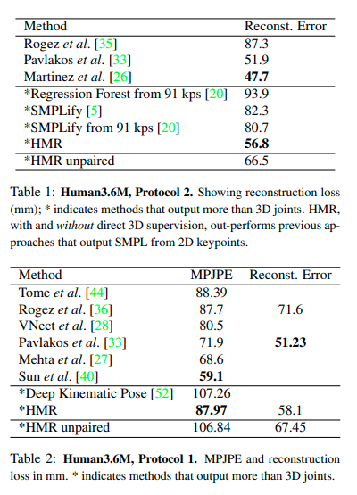
We report using several error metrics that are used for evaluating 3D joint error. Most common evaluations report the mean per joint position error (MPJPE) and Reconstruction error, which is MPJPE after rigid(경직된) alignment of the prediction with ground truth via Procrustes Analysis .
Human3.6M
We evaluate on two common protocols. The first, denoted P1, is trained on 5 subjects (S1, S5, S6, S7, S8) and tested on 2 (S9, S11).
The second protocol, P2, uses the same train/test set, but is tested only on the frontal camera (camera 3) and reports reconstruction error.
HMR is competitive with recent state-of-the-art methods that only predict the 3D joint locations.
MPI-INF-3DHP
The test set of MPI-INF-3DHP consists of 2929 valid frames from 6 subjects performing 7 actions.
Ground truth 3D annotations have some noise. In addition to MPJPE, we report the Percentage of Correct Keypoints (PCK) thresholded at 150mm and the Area Under the Curve (AUC) over a range of PCK thresholds.

4.2 Human Body Segmentation
The images have labels for six body part segments and the background.
Note that LSP contains complex poses of people playing sports and no ground truth 3D labels are available for training. We do not use the segmentation label during training either.
We also report results on foreground-background segmentation. Note that the part definition segmentation of the SMPL mesh is not exactly the same as that of annotation; this limits the best possible accuracy to be less than 100%.
Results are shown in Table 4. Our results are comparable to the SMPLify oracle, which uses ground truth segmentation and keypoints as the optimization target.
4.3 Without Paired 3D supervision
So far we have used paired 2D-to-3D supervision, i.e. L_3D whenever available.
Here we evaluate a model trained without any paired 3D supervision.
A model trained with neither the paired 3D supervision nor the adversarial loss produces monsters with extreme shape and poses.
5. Conclusion
In this paper we present an end-to-end framework for recovering a full 3D mesh model of a human body from a single RGB image.
We parameterize the mesh in terms of 3D joint angles and a low dimensional linear shape space, which has a variety of practical applications.
Our results without using any paired 3D data are promising since they suggest that we can keep on improving our model using more images with 2D labels, which are relatively easy to acquire, instead of ground truth 3D, which is considerably more challenging to acquire in a natural setting.
- 학부생 때 만든 것이라 오류가 있거나, 설명이 부족할 수 있습니다.
Uploaded by N2T
'Paper Summary' 카테고리의 다른 글
| Graph Attention Networks, ICLR’18 (0) | 2023.03.26 |
|---|---|
| GaAN: Gated Attention Networks for Learning on Large and Spatiotemporal Graphs, UAI’18 (0) | 2023.03.26 |
| Learning Actor Relation Graphs for Group Activity Recognition, CVPR’19 (0) | 2023.03.26 |
| Mesh Graphormer, ICCV’21 (0) | 2023.03.26 |
| Actor-Transformers for Group Activity Recognition, CVPR’20 (0) | 2023.03.26 |